This post will cover the concepts of image processing to generate and display image disparity or depth of field. This topic has been covered in earlier posts in regards to anaglyph imaging and OpenCV disparity mapping. The purpose of this post is to expand on this topic by demonstrating some features and limitations. Let’s start by leaving flatland.

Flatland & the 4th Dimension – Carl Sagan

This image is of a stereo card from the Missouri History Museum that is dated between 1914 and 1918 which depicts a wasteland as a result from World War 1. It is available as a free media repository from Wikimedia Commons, https://commons.wikimedia.org/wiki/File:%22Desolate_Waste_on_Chemin_des_Dames_Battlefield,_France.%22.jpg

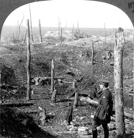
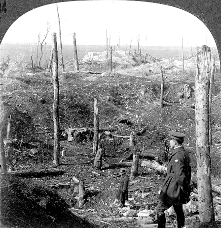
Stereo cards were a common technique during early photography to give the viewer the illusion of depth. They peaked in popularity between 1902 and 1935. The University of Washington contains a digital collection of these artifacts, https://content.lib.washington.edu/stereoweb/index.html

I used a different method for processing images into depth with OpenCV from the example image above. First, the stereo card was split into 2 separate images and tonal qualities were applied which gave the best contrast. The following script requires that both images have matching dimensions.

import numpy as np
import cv2 as cv
from matplotlib import pyplot as plt

imageLeft = cv.imread('resized_v18834-right.png', 0)
imageRight = cv.imread('resized_v18834-left.png', 0)

# Using StereoSGBM
# Set disparity parameters. Note: disparity range is tuned according to
#  specific parameters obtained through trial and error.
win_size = 2
min_disp = -4
max_disp = 9
# num_disp = max_disp - min_disp  # Needs to be divisible by 16
num_disp = 32  # Needs to be divisible by 16
stereo = cv.StereoSGBM_create(
    minDisparity=min_disp,
    numDisparities=num_disp,
    blockSize=7,
    uniquenessRatio=5,
    speckleWindowSize=5,
    speckleRange=5,
    disp12MaxDiff=2,
    P1=8 * 3 * win_size ** 2,
    P2=32 * 3 * win_size ** 2,
)
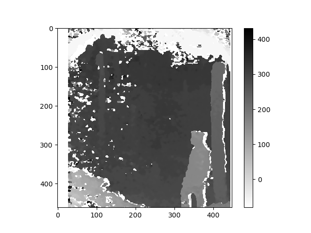
disparity_SGBM = stereo.compute(imageLeft, imageRight)
cmap_reversed = plt.cm.get_cmap('gray_r')
plt.imshow(disparity_SGBM, cmap_reversed)
plt.colorbar()

plt.savefig("ver11_v18834-depth.png")

This created the following grayscale depth map image.

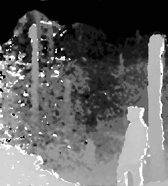
I then manually edited the image in an attempt to reduce holes, pitting, and other noise while adding more contrast to the overall image, here is the result.

Some images that lack a secondary viewpoint can have a depth map layer manually created using GIMP. This technique is demonstrated in this video.

I applied a similar technique with this image. The rgb image is on the left while the grayscale depth map image is on the right.

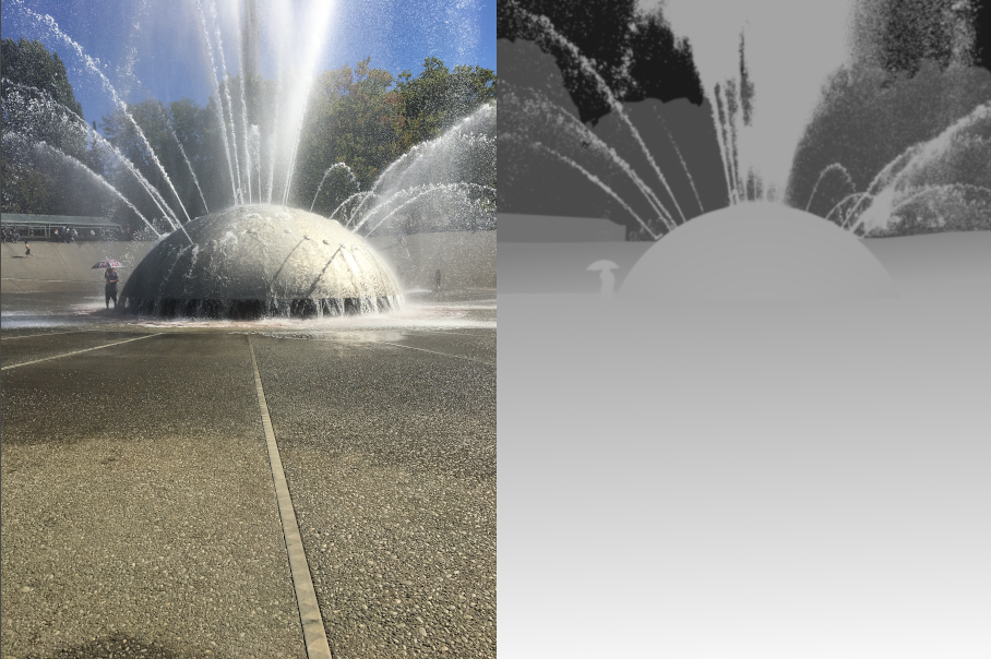
Using GIMP, I generated a series of images by changing the amount of map and displace values. This group of images was then generated into a video with FFMPEG to give a sense of depth and motion.

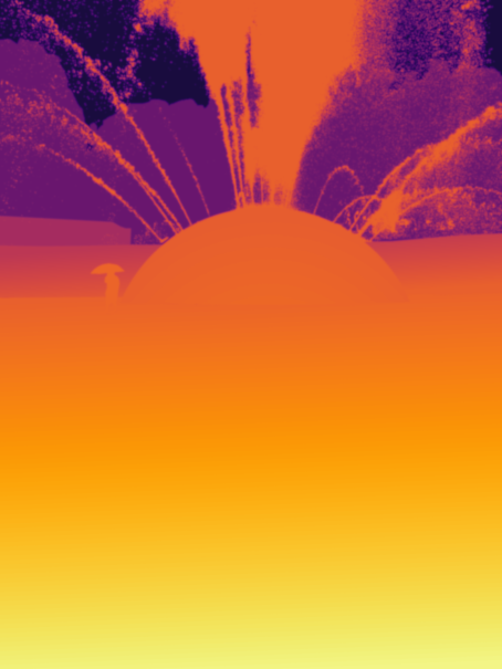
The grayscale depth map image was further processed to create a false color image with the inferno scale using this script.

import matplotlib.pyplot as plt
import numpy as np
import cv2

image = cv2.imread('IMG_1675_Depth_Blurred.png', 0)
colormap = plt.get_cmap('inferno')
heatmap = (colormap(image) * 2**16).astype(np.uint16)[:,:,:3]
heatmap = cv2.cvtColor(heatmap, cv2.COLOR_RGB2BGR)
cv2.imwrite('IMG_1675_Color_Depth_Blurred.png',heatmap)

I also applied this technique to panoramic images to generate an VR perspective using Google Street View by importing the resulting images. Here is an example video of rgb, grayscale depth, and false color depth.

Here is the 360 degree false color depth map.

Capturing images with a monocular camera presented challenges. There are a number of factors that will influence the final quality of the render, some of them being lens distortion, plane alignment, parallax bend, focus, and any image correction that might occur automatically. The following images were captured with an iPhone app call CrossCam, https://apps.apple.com/us/app/crosscam/id1436262905. Unfortunately, as of this writing Apple has recently announced that they will be removing apps that have not received updates longer than 2 years, so I can’t say if Kevin Anderson’s work will still be available. Here’s a link to the story.

https://www.theverge.com/2022/4/23/23038870/apple-app-store-widely-remove-outdated-apps-developers

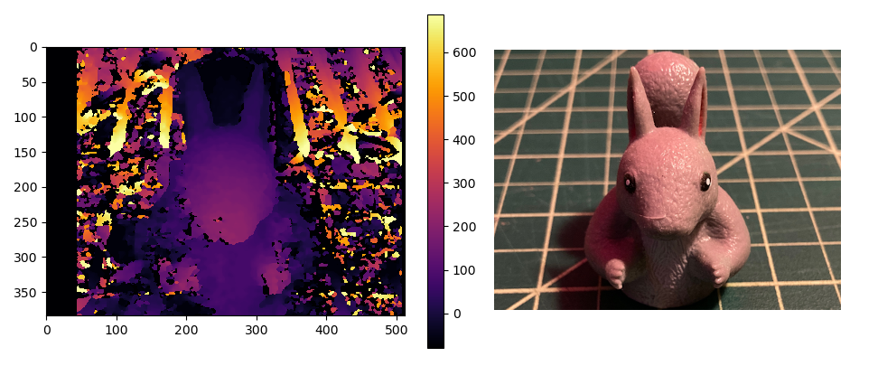
At any rate, the following image depth map was created which resulted in a large amount of noise.

This paper details much of the requirements facing accurate depth map generation from stereo image sets.  These same topics were pointed out in this post, https://stackoverflow.com/questions/36172913/opencv-depth-map-from-uncalibrated-stereo-system

https://images.autodesk.com/latin_am_main/files/stereoscopic_whitepaper_final08.pdf

Taking all of these into account, it is entirely possible to use inexpensive ESP32-Cam modules to generate depth map images, provided they are aligned and set correctly.

This process performs depth map estimation using MIDaS, details about MIDAS can be found here, https://pytorch.org/hub/intelisl_midas_v2

There is much more that can be covered on this topic which is beyond digestible in one sitting. Pun intended, this topic is deep.