This post will revisit a topic which has been covered in earlier posts, but with some enhancements.  This earlier post used python to visualize a radio sweep, https://www.cloudacm.com/?p=3209. The method was specific to the SDR hardware and the rtl_power command to generate a dataset that was then processed with python to generate a plot.  This post will expand on the visualization by using python to generate varied plot types to help in understanding the radio signals observed.  The previous post was limited to the SDR hardware.  In this post, the processed datasets will be the focus with an unfixed approach to the data sources.

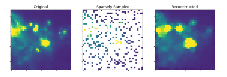
This link provided some footing on the python method, https://docs.astropy.org/en/stable/convolution/index.html.  What is interesting about the method is its ability to fill in the blanks of a sparse dataset and the results closely matching the higher resolution control.

This was applied to RSSI readings taken in an area to generate a heat map of the signal coverage.  Here is the python code used.

import matplotlib.pyplot as plt
import numpy as np
from scipy.interpolate import Rbf  # radial basis functions

# x y arrays
x = [1, 3, 4, 4, 5, 6, 8, 9, 10, 10, 11, 12, 15, 16, 17, 19, 19, 20]
y = [5, 15, 10, 18, 3, 16, 8, 10, 5, 18, 15, 9, 8, 16, 18, 4, 14, 9]
z = [-42, -53, -44, -58, -28, -48, -62, -62, -44, -69, -66, -64, -49, -67, -72, -36, -55, -40]
# this made it click
# https://stackoverflow.com/questions/65652769/interpolation-scatter-plot
# z = [1]*len(x)

#RBF Func
rbf_fun = Rbf(x, y, z, function='linear')

x_new = np.linspace(0, 20, 81)
y_new = np.linspace(0, 18, 82)

x_grid, y_grid = np.meshgrid(x_new, y_new)
z_new = rbf_fun(x_grid.ravel(), y_grid.ravel()).reshape(x_grid.shape)

plt.pcolor(x_new, y_new, z_new);
plt.plot(x, y, 'o');
plt.xlabel('x'); plt.ylabel('y');
plt.title('RBF Linear interpolation');
plt.show();

The x and y values were points derived from a floor plan, while the z values were RSSI signal readings made using the AirPort Utility on an iPhone.  The AirPort Utility can be set to measure signal strength and display the values by enabling the Wi-Fi Scanner option in the app settings.  This process requires manual data point entry, which can be tedious and prone to error on a large and repetitive scale.  However, for the purposes of a demonstration it can prove to be valuable.  Here are the results of the plot compared to the sparse readings.

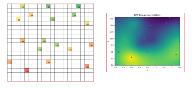
The interpolated plot fills in the blanks to give a smoother appearance of the radio coverage.  These heatmaps can be generated using commercial software.  However, the licensing costs often keep it out of the reach of those that may have casual or occasional use for it.

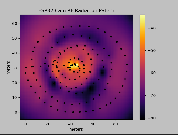
Another case use would be radio location.  In this example, an area was surveyed with the ESP32-Cam data logger that was discussed in this post, https://www.cloudacm.com/?p=3681.  The data logger captured the x and y values as GPS coordinates, while the z values are the RSSI values.  These RSSI values were captured from another ESP32-Cam module acting as a beacon, it was originally a time lapse camera from this post, https://www.cloudacm.com/?p=4036.  The beacon was encircled by the data logger with the data logger always facing in the same direction towards the beacon.  The plot closely matches a typical radio pattern along its horizontal axis.

Here is the python code used with the included datasets.

from scipy.interpolate.rbf import Rbf  # radial basis functions
import matplotlib.pyplot as plt
import numpy as np

fig = plt.figure(facecolor='silver')

# Longitude values 
y = [30.48, 31.47, 32.26, 32.65, 30.93, 29.70, 29.89, 28.12, 26.99, 27.33, 28.56, 30.48, 33.64, 35.51, 36.64, 36.00, 34.18, 31.91, 29.45, 26.64, 24.13, 22.36, 22.31, 23.39, 25.51, 27.82, 30.63, 33.93, 36.98, 39.45, 41.56, 43.63, 44.52, 42.55, 39.40, 35.95, 32.21, 27.23, 22.75, 18.86, 16.60, 16.05, 17.38, 20.04, 23.64, 27.68, 32.50, 34.23, 35.26, 40.38, 43.24, 45.36, 44.91, 42.40, 38.95, 34.96, 30.78, 26.59, 22.21, 19.70, 16.05, 13.20, 12.46, 13.94, 16.40, 19.65, 23.69, 28.27, 32.90, 36.79, 40.48, 44.08, 47.18, 50.97, 52.40, 51.76, 50.23, 47.47, 43.09, 38.22, 33.64, 28.96, 24.23, 19.50, 15.32, 11.67, 8.82, 6.70, 5.71, 5.32, 6.21, 7.73, 10.34, 13.84, 17.58, 21.87, 26.54, 30.98, 35.75, 41.17, 44.08, 47.67, 51.41, 54.12, 56.14, 57.57, 58.11, 58.41, 57.96, 56.53, 54.22, 51.07, 47.67, 42.94, 38.26, 32.40, 27.63, 22.60, 17.97, 13.49, 9.50, 6.45, 4.83, 2.56, 0.98, 0.64, 0.15, 0.00, 0.34, 1.63, 3.79, 6.55, 9.65, 13.30, 17.58, 21.82, 26.45, 30.29, 30.93, 31.17, 31.27, 31.52, 31.71, 31.52, 31.86]

# Latitude Values
x = [39.48, 40.19, 41.42, 43.57, 46.74, 47.97, 47.86, 47.97, 46.13, 42.95, 39.48, 37.53, 38.35, 39.58, 43.26, 47.15, 50.22, 51.65, 51.75, 51.95, 47.86, 43.87, 39.07, 35.39, 32.52, 29.56, 27.82, 28.23, 28.94, 30.78, 34.36, 40.30, 45.92, 51.14, 55.43, 57.89, 58.40, 57.17, 54.31, 49.70, 44.59, 40.70, 36.20, 30.78, 27.20, 24.03, 24.24, 24.85, 26.08, 30.37, 37.02, 45.41, 52.67, 59.42, 63.92, 68.11, 69.44, 67.91, 64.84, 60.34, 57.27, 50.42, 44.59, 38.25, 30.78, 25.36, 21.89, 18.61, 17.08, 17.39, 19.84, 23.32, 28.23, 34.36, 42.03, 49.70, 56.86, 63.92, 69.55, 74.15, 76.19, 76.50, 75.17, 72.92, 70.26, 65.25, 60.14, 54.10, 47.97, 41.11, 34.26, 28.23, 23.11, 17.69, 13.19, 9.82, 7.26, 5.42, 5.42, 6.55, 8.18, 10.84, 15.65, 21.37, 27.31, 33.75, 40.50, 48.27, 56.15, 64.23, 70.36, 75.78, 81.00, 84.78, 88.26, 90.00, 89.80, 88.26, 86.11, 83.35, 79.77, 75.27, 71.59, 65.97, 59.73, 53.39, 48.17, 42.14, 35.28, 28.43, 22.50, 16.87, 12.27, 8.49, 4.70, 2.05, 0.00, 0.31, 6.55, 13.40, 20.45, 27.31, 34.06, 41.22, 44.49]

# Sensor Readings 
z = [-38, -37, -43, -50, -49, -49, -48, -51, -55, -54, -48, -49, -49, -51, -53, -61, -59, -53, -51, -53, -54, -56, -57, -59, -62, -52, -55, -55, -61, -58, -60, -61, -60, -56, -57, -55, -57, -55, -59, -60, -63, -61, -58, -55, -53, -52, -53, -52, -54, -56, -59, -63, -63, -66, -66, -66, -70, -81, -71, -75, -81, -76, -76, -70, -70, -81, -70, -74, -69, -65, -67, -64, -75, -74, -71, -73, -76, -74, -70, -70, -64, -63, -64, -63, -69, -70, -70, -76, -68, -66, -68, -64, -66, -64, -60, -58, -58, -57, -59, -62, -62, -59, -61, -62, -63, -65, -67, -68, -68, -68, -68, -66, -66, -63, -62, -65, -64, -65, -63, -64, -66, -67, -66, -66, -70, -71, -66, -65, -67, -65, -64, -68, -61, -63, -61, -59, -58, -58, -59, -64, -65, -51, -49, -38, -29]

rbf_adj = Rbf(x, y, z, function='linear')

# horizontal range
y_fine = np.linspace(-5, 66, 82)
# vertical range
x_fine = np.linspace(-5, 95, 81)


x_grid, y_grid = np.meshgrid(x_fine, y_fine)

z_grid = rbf_adj(x_grid.ravel(), y_grid.ravel()).reshape(x_grid.shape)

# https://matplotlib.org/stable/tutorials/colors/colormaps.html
# plt.pcolor(x_fine, y_fine, z_grid);
# plt.pcolor(x_fine, y_fine, z_grid, cmap=plt.cm.autumn);
plt.pcolor(x_fine, y_fine, z_grid, cmap=plt.cm.inferno);
# plt.pcolor(x_fine, y_fine, z_grid, cmap=plt.cm.hot);


plt.plot(x, y, '.k');
plt.xlabel('meters'); plt.ylabel('meters'); plt.colorbar();
plt.title('ESP32-Cam RF Radiation Patern');

# plt.show()
fig.savefig('Plot_RF-Pattern_Meters1.png', facecolor=fig.get_facecolor()) 

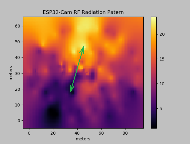
The next plot contains z values that were detected networks in the area.  It should be noted that the orientation of the ESP32-Cam module that was taking the readings was maintained toward the beacon.  This is an important factor, as seen in this plot, because the direction of the networks detected becomes visible.

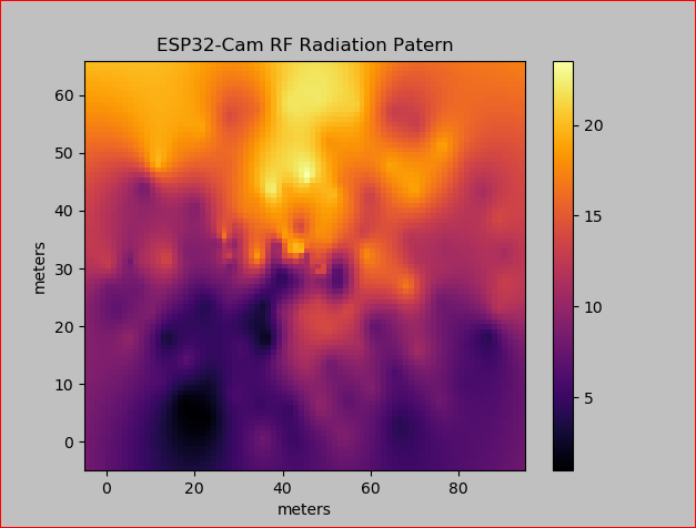
The bright yellow and dark purple areas establish the linear path toward the network sources.  The following illustration shows the direction in green.

The original intention was to plot the beacon’s radiation pattern.  It was a welcomed surprise to be able to plot the direction of these networks.  However, it should be noted that the interpolation method requires readings to be well spaced.  The following plots demonstrate the limitations inherent to interpolation.

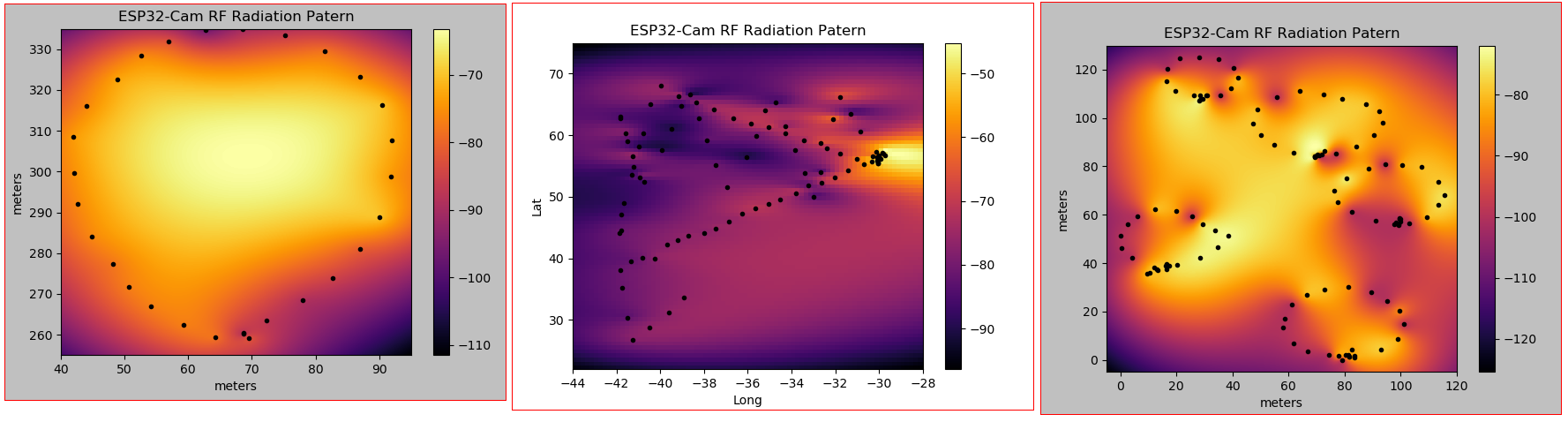The resulting interpolated data is incorrect, so be aware of the context when using this method.

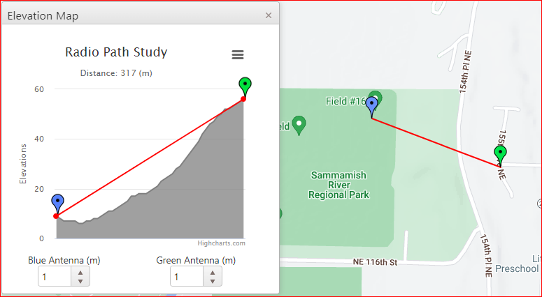
The following were some useful resources found during the research of this topic.  RF Line of Sight, https://www.scadacore.com/tools/rf-path/rf-line-of-sight/.

DragonOS LTS an out-of-the-box Lubuntu 20.04 based x86_64 operating system for anyone interested in software defined radios but were too scared to ask, https://sourceforge.net/projects/dragonos-lts/.

Array sensing uses.

Data sampling with SDR hardware, the ability to record SDR data for post analysis.