SDR Data Processing
In the last post, https://www.cloudacm.com/?p=4136, there was a lead in on the topic of capturing the data from SDR hardware using GQRX. This post was also mentioned, https://www.cloudacm.com/?p=3209. In this post, these topics will be revisited with some greater detail and enhancement.
The first item covered here will be IQ data captured using GQRX. When using GQRX with SDR hardware, it’s not always convenient to view the data live. This has been the case during my field work, with the elements being a factor on how cumbersome live viewing can be. Fortunately, the steps to capture SDR data in GQRX is rather simple. For those of you new to GQRX, more information about GQRX can be found here, https://gqrx.dk/doc/practical-tricks-and-tips
The concept of IQ data is complex, details are presented in this post, https://www.allaboutcircuits.com/textbook/radio-frequency-analysis-design/radio-frequency-demodulation/understanding-i-q-signals-and-quadrature-modulation/. To capture IQ data, start by attaching the SDR hardware and running GQRX. From the menu bar, select Tools > I/Q recorder, or press Ctrl+I. Set the path where to save the IQ data stream and press record, that’s it. This video demonstrates the process, here is the FFMpeg command used to capture the desktop video.
ffmpeg -video_size 1920x1080 -framerate 10 -f x11grab -i :0.0+1920,0 GQRX_IQRecord.mp4
With the captured file, gqrx_20220830_064000_99500000_1800000_fc.raw, there are some key pieces of information contained in the file name. Here is a breakdown of that information.
GQRX – This is the program used to capture the file.
20220830 – This is the date of the capture, in the YYYYMMDD format.
064000 – This is the timestamp of the capture, in HHMMSS format.
99500000 – This is the center frequency of the capture, 99.5 Mhz.
18000000 – This is the sample rate, 1.8M samples per second.
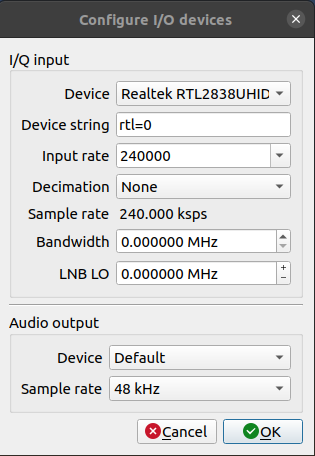
The data file can be replayed in GQRX by entering the I/Q input parameters. Here is an example of that parameter.
file=/path/to/your/file,freq=100e6,rate=1e6,repeat=true,throttle=true.
Here is a breakdown of that parameter string which we will use for the previous sample.
file=/home/local/Desktop/gqrx_20220830_064000_99500000_1800000_fc.raw – Defines file input with full path
freq=995e5 – Defines center frequency, here it’s set to 99,500,000 Hz or the standard 99.5 Mhz
rate=1.8e6 – This defines the sample frequency, how often each sample was taken during recording. Here it’s set to 18,000,000 or 18Mhz
repeat=true – This tell GQRX whether to play the sample once or loop play
file=/home/local/Desktop/gqrx_20220830_064000_99500000_1800000_fc.raw,freq=995e5,rate=1.8e6,repeat=true
Be sure to turn your volume down, something bumped my volume to max and I got someone’s attention, nearly dropped my coffee. Here is a video of the process of importing the IQ data using the parameter above, again with this FFMpeg command.
ffmpeg -video_size 1920x1080 -framerate 10 -f x11grab -i :0.0+0,0 GQRX_IQReplay.mp4
The data file is rather large, be mindful of the sample rate if space is a concern. When setting the SDR hardware options, changing the input rate will save space at the cost of resolution. The sample rate above is the same as the input rate.
Having the IQ data file available later gives all the benefits of a live capture, but in the comfort of your home. The post analysis can be quite extensive, here are a series of posts that delve much further into SDR.
Using SDR to Build a Trunk Tracker – Police, Fire, and EMS Scanner
https://www.blackhillsinfosec.com/using-sdr-to-build-a-trunk-tracker-police-fire-and-ems-scanner/
Using IQ Files
https://www.pe0sat.vgnet.nl/sdr/sdr-software/using-iq-files/
Capture and decode FM radio
https://witestlab.poly.edu/blog/capture-and-decode-fm-radio/
FM HD Radio decode from I/Q files
https://pclover.net/FM-HD-Radio-decode-iq-file.html
There are other SDR tools that can capture data from the RTL hardware, one of these is RTL-433. This command will capture the IQ data.
rtl_433 -w /home/local/Desktop/Sample.cf32
To read from the file use this command.
rtl_433 -r /home/local/Desktop/Sample.cf32
Note that rtl_433 supports these file types: CU8, CS16, CF32 I/Q data, U16 AM data (built-in). Only CF32 has IQ data and is thus readable form GQRX, so be aware if you intend to view the readings later.
From our sampling, we are able to open it in GQRX. Adjusting the rate can be used to slow down the playback, which can reveal missed items in a live real-time scenario. Here is the GQRX parameter string to playback the rtl_433 sample at a slower rate.
file=/home/local/Desktop/Sample.cf32,freq=433e6,rate=1e5,repeat=true
This command was used to help aid in how the sample was created with frequency and sample rates included in the IQ file. Below is the GQRX parameters to allow for playback.
rtl_433 -f 146952e3 -M raw -s 18e5 -w /home/local/Desktop/rtl_433_146952e3_18e5_20220830_054500.cf32
file=/home/local/Desktop/rtl_433_146952e3_18e5_20220830_054500.cf32,freq=146952e3,rate=18e5,repeat=true,throttle=true
This topic, https://www.cloudacm.com/?p=3209, captured data using the rtl_power command. The original processing method was fairly simple. This has been expanded to use plotly to generate a more customizable waterfall. Here are a series of commands used to generate a waterfall of a 10 minute sweep.
rtl_power -f 156M:158M:3.125k -i 1 -e 10m RTL_RF_Logfile_202208300725.csv
cut -d"," -f7- RTL_RF_Logfile_202208300725.csv > RTL_RF_Logfile_Raw_202208300725.csv
python3 RTL_RF_Logfile_Raw_202208300725.py
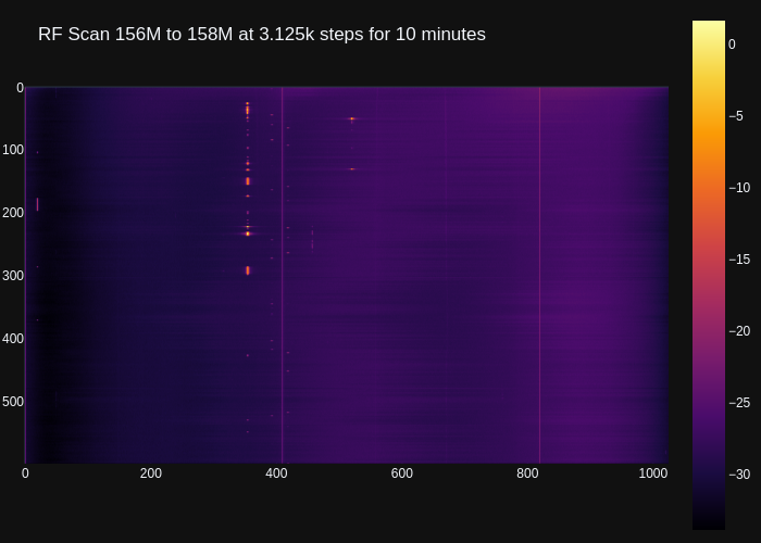
In order to use it, the original csv file need to be massaged by removing leading columns that did not contain the actual RF db readings, done simply with the cut command. Here is the python code used.
import plotly.express as px
from numpy import genfromtxt

data = genfromtxt('/home/local/Desktop/RTL_RF_Logfile_Raw_202208300725.csv', delimiter=',')

# ig = px.imshow(data, color_continuous_scale=px.colors.sequential.gray)
# https://plotly.com/python/builtin-colorscales/
# fig = px.imshow(data, color_continuous_scale=px.colors.sequential.Blackbody)
# fig = px.imshow(data, color_continuous_scale=px.colors.sequential.Plasma)
fig = px.imshow(data, color_continuous_scale=px.colors.sequential.Inferno, template="plotly_dark")

fig.update_layout(margin=dict(l=2, r=2, b=2, t=2), coloraxis_showscale=True, plot_bgcolor="Black")
fig.update_layout(title_text='RF Scan 156M to 158M at 3.125k steps for 10 minutes',title_y=0.95)
fig.update_xaxes(showticklabels=True).update_yaxes(showticklabels=True)
# fig.show()

fig.write_image("/home/local/Desktop/RTL_RF_Logfile_Raw_202208300725.png")

# Command - python3 file2.py
# Source - https://plotly.com/python/heatmaps/
# Color Scales - https://plotly.com/python/builtin-colorscales/

# https://plotly.com/python/imshow/
# https://pypi.org/project/plotly-express/
# https://www.cloudacm.com/?p=2674
# https://plotly.com/python/plotly-express/
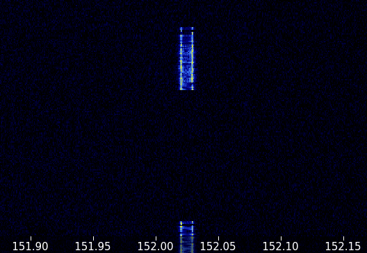
This post contains details about POCSAG, https://www.sigidwiki.com/wiki/POCSAG. This post shows how to use rtl_fm and multimon-ng to decode the POCSAG radio signal, https://lokcon.me/2019/06/18/rtl-sdr-pocsag. I used the following command after isolating the POCSAG baud rate. The text file contained some readable strings, most were unreadable though.
rtl_fm -M fm -f 152e6 -s 22050 | multimon-ng -t raw -a POCSAG1200 /dev/stdin > PocSagDecode.txt
tail -f PocSagDecode.txt
I then did a rtl_power sweep to plot the transmissions over a 10 minute period. It appears that these transmissions are from the same source. The decoded signals gave details for areas throughout the region, so this would suggest that this transmitter is part of a group of repeaters to provide wider coverage. Here are resulting plots from rtl_power and GQRX.
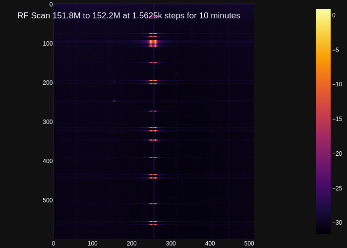
Here are the commands to generate the rtl_power plot with python.
rtl_power -f 151.8M:152.2M:1.5625k -i 1 -e 10m RTL_RF_Logfile_202211240700.csv
cut -d"," -f7- RTL_RF_Logfile_202211240700.csv > RTL_RF_Logfile_Raw_202211240700.csv
python3 RTL_RF_Logfile_Raw_202211240700.py
With the dataset, other processing tools and methods can be used to visualize the readings from rtl_power. It’s quite amazing the amount of resources and uses of the RTL SDR there are. The following video demonstrates how to use SDR for GPS readings.